Remainder Theorem Visualized with a Cubic Polynomial
Grades 10-11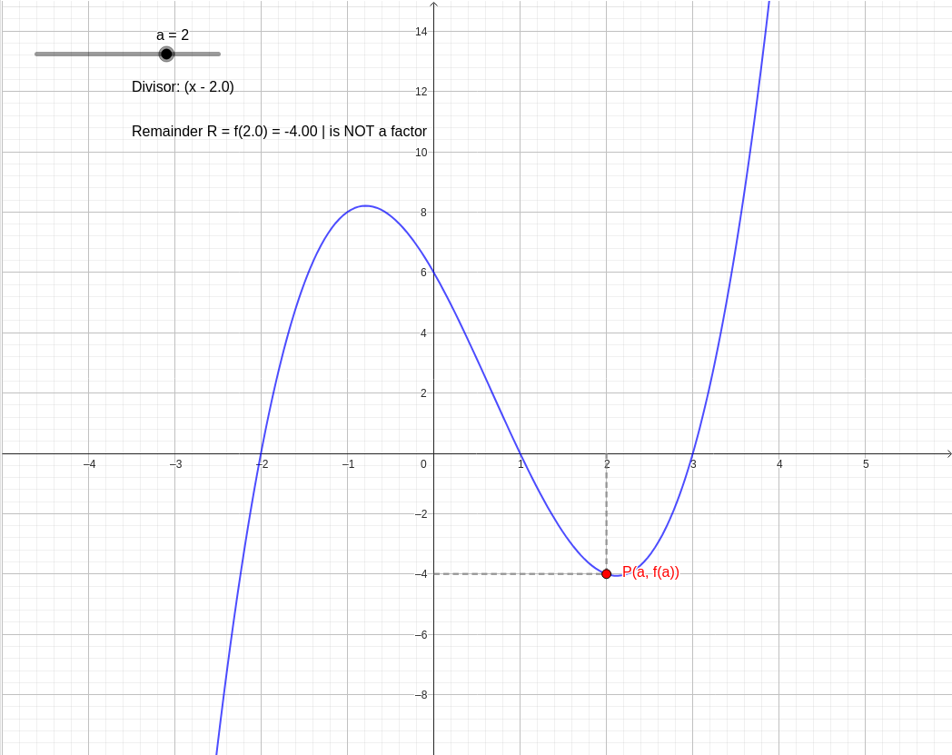
Question: explain and plot this: The Interactive Slider Concept: "The Remainder Tracker" To visualize this, we can plot a cubic polynomial on a coordinate grid, for example: y = f ( x ) = x 3 − 2 x 2 − 5 x + 6 y=f(x)=x 3 −2x 2 −5x+6 We then provide a draggable slider for a a (representing the divisor x − a x−a ), sliding from − 3 −3 to 4 4 . What the Applet Displays on the Screen: The Cubic Curve: y = x 3 − 2 x 2 − 5 x + 6 y=x 3 −2x 2 −5x+6 plotted in blue. The Slider: Controls the value of a a . A Vertical Tracker Line: A dashed line at x = a x=a extending to meet the curve at point P ( a , f ( a ) ) P(a,f(a)) . A Horizontal Remainder Line: A dashed line extending from point P P to the y y -axis to show its height (the remainder R R ). A Live Equation Box: Updates dynamically: Divisor: ( x − a ) ⟺ Remainder R = f ( a ) Divisor: (x−a)⟺Remainder R=f(a) What Students See by Dragging the Slider As the student drags the slider to adjust a a , they watch the tracker point ride along the cubic curve and observe how the remainder changes [3]: code Code y | P(a, f(a)) _ _ _ _ _ _ _ _ _ _|_ _ _ _ * (The Remainder is the height!) | | / | | / | | / -|- - - - - - - - - -|- - -|- - - - - - - x | a (The Divisor x - a) | Case 1: When a = 2 a=2 (The General Remainder) The Graph: The slider is set to a = 2 a=2 . The vertical tracker line stops at P ( 2 , − 4 ) P(2,−4) below the x x -axis. The horizontal line points to − 4 −4 on the y y -axis. The Live Equation Box: When f ( x ) is divided by ( x − 2 ) ⟹ Remainder R = f ( 2 ) = − 4 When f(x) is divided by (x−2)⟹Remainder R=f(2)=−4 The Lesson: Students see that the remainder is simply the y y -coordinate of the graph at x = a x=a . Because the remainder is not 0 0 , ( x − 2 ) (x−2) is not a factor of the polynomial. Case 2: When a = 3 a=3 (The Factor Theorem) The Graph: The student slides a a to exactly 3 3 . The tracker point P ( 3 , 0 ) P(3,0) lands perfectly on the x x -axis (the x x -intercept). The horizontal line points to 0 0 on the y y -axis. The Live Equation Box: When f ( x ) is divided by ( x − 3 ) ⟹ Remainder R = f ( 3 ) = 0 When f(x) is divided by (x−3)⟹Remainder R=f(3)=0 The Lesson: Because the remainder is exactly 0 0 , the Factor Theorem states that ( x − 3 ) (x−3) is a factor of f ( x ) f(x) . The student visually connects "being a factor" to "crossing the x x -axis." Case 3: Scanning for other factors If the student continues sliding, they will watch the point cross the x x -axis at two other positions: At a = 1 ⟹ P ( 1 , 0 ) ⟹ ( x − 1 ) a=1⟹P(1,0)⟹(x−1) is a factor. At a = − 2 ⟹ P ( − 2 , 0 ) ⟹ ( x + 2 ) a=−2⟹P(−2,0)⟹(x+2) is a factor. By the end of the simulation, they see that the fully factorized cubic is: f ( x ) = ( x − 3 ) ( x − 1 ) ( x + 2 ) f(x)=(x−3)(x−1)(x+2) Why this is a Game-Changer for HKDSE Paper 2 DSE Paper 2 frequently includes questions that show a sketch of a cubic curve crossing the x x -axis at three integer points (e.g., − 2 −2 , 1 1 , and 3 3 ) and ask you to identify the correct equation. Most students solve these slowly by substituting coordinates to set up simultaneous equations. If they interact with this slider, they will instantly recognize the shortcut: if the graph crosses at − 2 −2 , 1 1 , and 3 3 , the factors must be ( x + 2 ) (x+2) , ( x − 1 ) (x−1) , and ( x − 3 ) (x−3) , allowing them to solve the multiple-choice question in under 5 seconds.
In the HKDSE Mathematics (Compulsory Part), the Remainder Theorem and Factor Theorem are fundamental tools for handling polynomials. They bridge the gap between algebraic division and coordinate geometry.
1. The Remainder Theorem
When a polynomial
is divided by
, the remainder
is given by
.
Geometrically, if we look at the graph of
, the remainder
is simply the
-coordinate of the point on the curve where
.
2. The Factor Theorem
This is a special case of the Remainder Theorem. If
, then
is a factor of
.
On the graph, this occurs whenever the curve intersects the
-axis (the
-intercepts). At these points, the vertical height is zero, meaning there is "no remainder" left over after division.
3. Case Study:
In the interactive diagram below, you can move the slider to change the value of
(representing the divisor
).
-
General Remainder (e.g., ): As you slide to , the tracker point moves to . . Since the -coordinate is , the remainder is . Thus, is not a factor.
-
Finding Factors (The Factor Theorem): Observe what happens when the remainder tracker hits the -axis. This occurs at , , and . For , . This confirms that is a factor. By identifying all three intercepts, we can immediately determine the factorized form:
4. HKDSE Exam Shortcut (Paper 2)
In multiple-choice questions, you are often asked to identify the equation of a cubic graph from its intercepts.
- Locate the -intercepts .
- The factors must be .
- Match these to the options. (Note: Check the -intercept by calculating to ensure the leading coefficient is correct).
For our graph: Intercepts:
Factors:
-intercept check:
. This matches the constant term in
.