Integral of 1/(x^2020 + 46)

Grades 11-12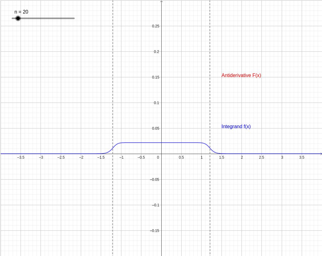

Question: \int \frac{1}{x^{2020} + 46} \, dx

The integral of the form

\int \frac{1}{x^n + a} \, dx

where

n

is a large even integer like 2020 is a classic example of a function that, while continuous and integrable, does not possess a simple antiderivative in terms of elementary functions (like polynomials, logs, or basic trig functions). To understand this integral, we examine the behavior of the integrand and the resulting area it accumulates.

1. Behavior of the Integrand

Let

f(x) = \frac{1}{x^{2020} + 46}

. We can identify two distinct regions based on the value of

x

The "Plateau" Region: When $|x|$ is small (specifically when $x^{2020} \ll 46$ ), the denominator is dominated by the constant $46$ . In this region, $f(x) \approx \frac{1}{46}$ . Because $2020$ is such a high power, this approximation remains extremely accurate for almost the entire interval $x \in (-1, 1)$ .
The "Decay" Region: When $|x|$ becomes larger than $1$ , the term $x^{2020}$ grows with extreme speed. The function $f(x)$ drops toward zero almost instantly. For example, at $x=1.1$ , $1.1^{2020}$ is a number with over 80 digits, making $f(x)$ effectively zero.

2. Geometry of the Integral

The integral

F(x) = \int f(x) \, dx

represents the "accumulated area" under this curve.

Near the origin, since $f(x) \approx \frac{1}{46}$ , the integral $F(x)$ behaves like a linear function: $F(x) \approx \frac{x}{46}$ . This is represented by the straight diagonal slope in the center of the diagram.
As $x$ passes the threshold $x \approx \pm 46^{1/2020} \approx \pm 1.002$ , the area stops accumulating because the integrand has dropped to zero. This causes the integral curve to "plateau" or flatten out into a horizontal line.

3. The Transition Point

The "corner" where the function switches from a constant height to a rapid decay occurs at

x = \pm \sqrt[n]{a}

. For

n=2020

and

a=46

, this value is roughly

1.0019

. In the visual model, you can adjust the exponent

n

to see how the "bell curve" becomes increasingly rectangular, resembling a "pulse" function as the power increases.

4. Mathematical Complexity

While we can express this integral using advanced mathematical tools like Hypergeometric Functions or as a finite sum of logarithms and arctangents using the roots of unity, the "2020" exponent would result in a sum with over 1,000 terms. Visually and practically, it is most useful to view this integral as a process that builds a nearly perfect linear ramp between

x = -1

and

x = 1

and then stays constant.

In the diagram below:

The blue curve represents the integrand $f(x)$ . Notice how "square" it becomes as you increase $n$ .
The red curve represents the integral $F(x)$ . It shows the transition from a linear ramp to a flat constant.
The dashed lines mark the critical boundaries where the function transitions.