Improper Integrals of 1/x^p: When They Converge

Grades 11-12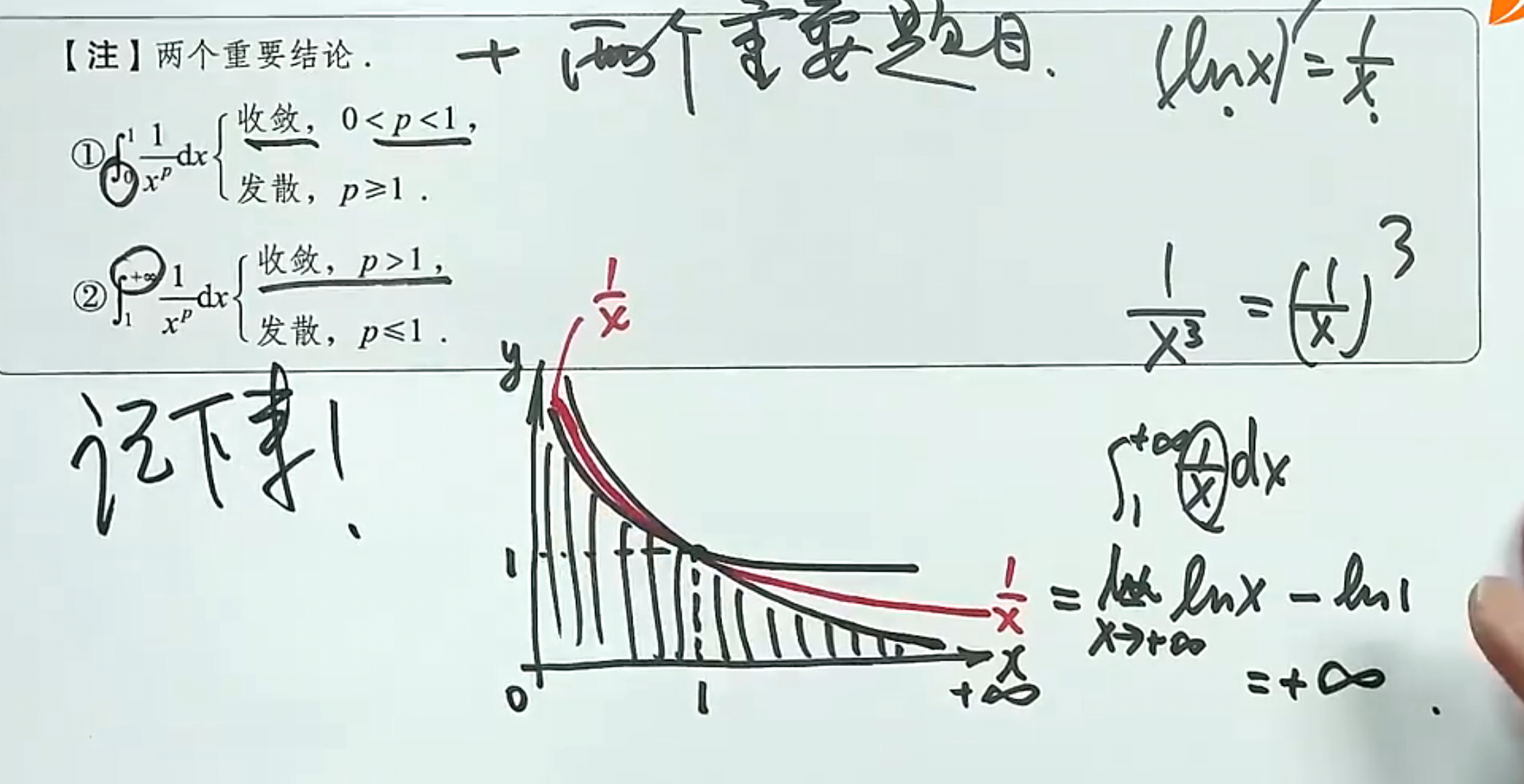

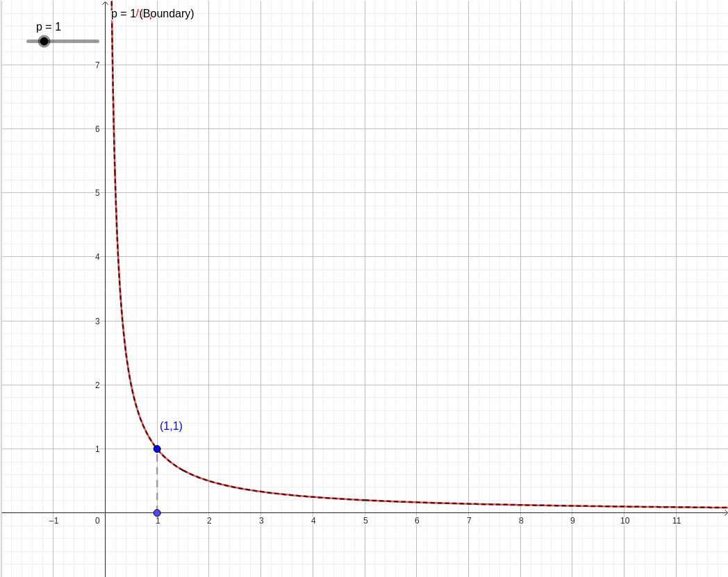
Question: Generate a graph of this function so I can more intuitively understand improper integrals.

Understanding the convergence of improper integrals through a graph comes down to watching how fast the curve approaches the

x

-axis "at infinity", and how fast it approaches the

y

-axis near a "singular point" (such as

x=0

We typically study functions of the form

y = \frac{1}{x^p}

. The exponent

p

controls how sharply the curve bends:

Infinite-interval improper integral (Type 1): Consider $\int_1^{+\infty} \frac{1}{x^p} dx$ . For the area at infinity to be finite, the function's values must decay "fast enough". $\begin{align*} \int_1^{+\infty} \frac{1}{x^p} dx &= \lim_{M \to +\infty} \left[ \frac{x^{1-p}}{1-p} \right]_1^M \quad (p \neq 1) \\ &\text{If } p > 1 \text{, the exponent is negative, so } M^{1-p} \to 0 \text{, and the area converges to } \frac{1}{p-1}. \\ &\text{If } p \le 1 \text{, the function decays too slowly, and the area diverges.} \end{align*}$
Singular-point integral (Type 2): Consider $\int_0^1 \frac{1}{x^p} dx$ . As $x \to 0$ , the function's values shoot up toward infinity. For the area near the $y$ -axis to be finite, the curve can't be too "steep". $\begin{align*} \int_0^1 \frac{1}{x^p} dx &= \lim_{\epsilon \to 0^+} \left[ \frac{x^{1-p}}{1-p} \right]_\epsilon^1 \quad (p \neq 1) \\ &\text{If } p < 1 \text{, the exponent is positive, so } \epsilon^{1-p} \to 0 \text{, and the area converges to } \frac{1}{1-p}. \\ &\text{If } p \ge 1 \text{, the function grows too fast, and the area diverges.} \end{align*}$

In the interactive model below, you can adjust the value of

p

with a slider:

The black dashed line represents the critical function $y = \frac{1}{x}$ ( $p=1$ ). At this critical value, the integral diverges on both sides.
The red curve represents your chosen $y = \frac{1}{x^p}$ .
Reference point (1,1): every function in this family passes through this point.
- As you increase p ( p > 1):
  - For $x > 1$ , the red curve stays below the black line with a "thinner" tail, so the right-side area converges.
  - For $x < 1$ , the red curve shoots higher than the black line, so the left-side area diverges.
- As you decrease p ( p < 1):
  - The situation flips completely: the left side converges, the right side diverges.

This "trade-off" relationship shows how the value of

p

controls how the area is distributed between the two sides.